Pest Forecasting: Simulating Population

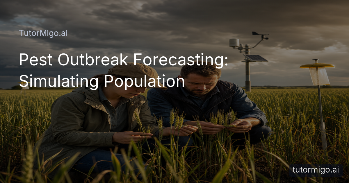
Why Pest Forecasting Starts With Population Dynamics

When a pest appears in a field, your hardest question is rarely what it is. The harder question is how quickly it will spread, where it will move next, and whether a treatment applied today will still be useful a week from now. Pest outbreak forecasting: simulating population dynamics gives agronomists a way to test those possibilities before damage becomes obvious.

A biological simulation represents a pest population as it changes over time. The model may track eggs, larvae, adults, survival, reproduction, and movement between fields. For example, a model for an aphid population can estimate how many winged adults leave a source field, how many settle on nearby plants, and how many reproduce under the expected temperature range.

The point is not to produce a perfect number. It is to compare plausible scenarios. If the model shows that a small population could double several times during a warm spell, scouting teams can inspect vulnerable fields sooner. If cooler nights slow development, the same teams may avoid an unnecessary blanket treatment and focus on monitoring instead.

Useful forecasting is less about predicting one certain future than identifying the decisions that become urgent under several likely futures.

How climate conditions change the forecast

Temperature, rainfall, humidity, wind, and crop growth all influence an outbreak. A warm period can shorten an insect’s development time, while heavy rain may suppress some exposed populations or move pathogens across plant surfaces. Wind can carry flying insects into new fields, and prolonged leaf wetness can create conditions favorable to fungal infection.

Forecasting software combines these inputs with field observations and historical records. A temperature-driven development model might estimate progress through a pest’s life cycle using accumulated heat units. In simplified form, daily development can be represented as $r(T)$, where $T$ is temperature and $r$ changes as conditions move toward or away from the pest’s preferred range. The model then adds those daily contributions across the season.

Climate scenarios are especially useful when conditions are unusual. Suppose a normally cool spring is followed by ten warm, humid days. One simulation may show earlier emergence of a beetle generation; another may show rapid disease progression after rain. Running both helps you distinguish a temporary spike from a pattern likely to persist.

Because weather forecasts carry uncertainty, strong systems show a range rather than a single confident outcome. That range tells you when to increase scouting and which observations would most improve the next forecast.

Modeling migration from field to field

Pests do not remain inside the boundaries of the field where they were first detected. A forecasting model can represent farms, hedgerows, waterways, and other landscape features as connected locations. It then estimates movement between them according to wind direction, distance, host availability, and the pest’s behavior.

Imagine that a trap network detects an increase in an invasive moth along the southern edge of a growing region. A migration model can test whether prevailing winds are likely to carry adults north, whether suitable crops form a continuous path, and how long eggs might take to hatch after arrival. The result may identify two fields that deserve immediate inspection even though their own traps remain quiet.

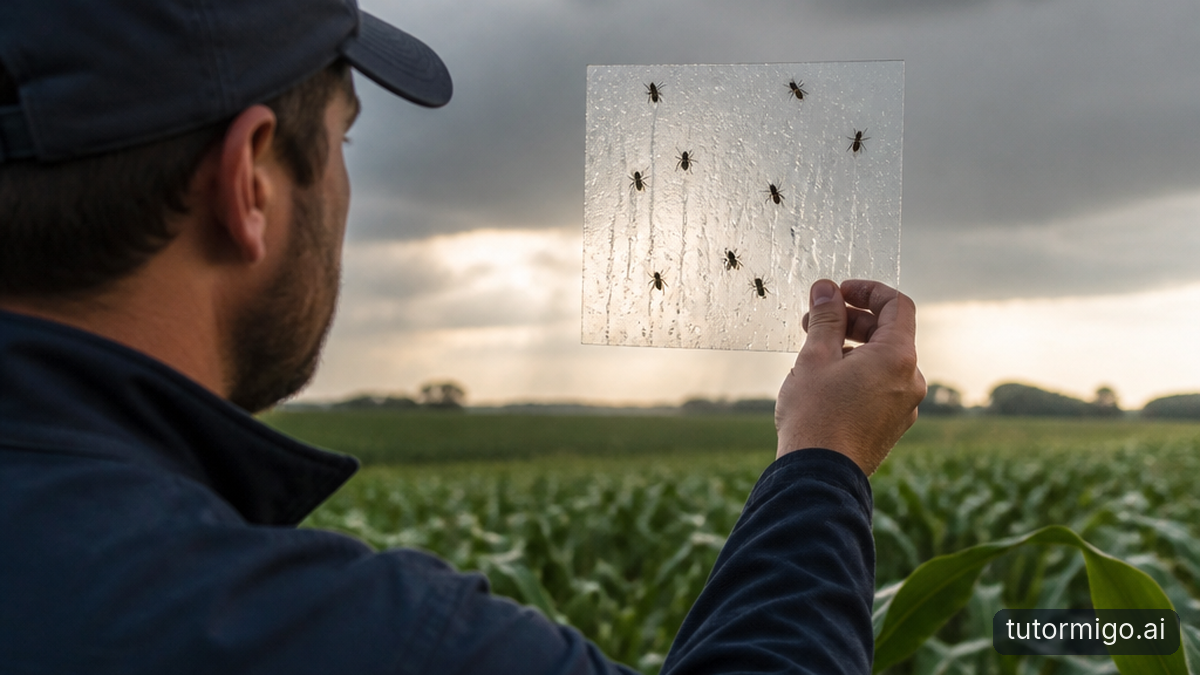
These models are most useful when paired with a clear sampling plan. Traps placed only in the center of a farm may miss an advancing edge. Adding sensors along boundaries, roads, or downwind margins can reveal movement earlier. Field crews can then compare predicted hotspots with actual counts and update the model.

Migration forecasts also support coordination. Neighboring growers may choose synchronized monitoring or treatment windows when a pest crosses property lines. That approach is more targeted than asking every farm to respond in the same way, regardless of local risk.

Simulating crop disease progression

Disease models follow a different chain of events from insect models, although the two can interact. A plant pathogen may need a susceptible host, a source of inoculum, moisture, and a suitable temperature window. The model estimates when infection can begin, how long symptoms take to appear, and how quickly spores or bacteria can reach new tissue.

For a fungal disease, the simulation might begin with spores present after an earlier infection. Rain splashes some spores onto nearby leaves, while wind carries others farther. If leaves remain wet long enough, a proportion may germinate. After an incubation period, new lesions produce more inoculum. Repeating that cycle shows why a field can move from scattered symptoms to serious damage surprisingly quickly.

Insect activity can raise the risk further. A pest that wounds leaves or feeds on plant tissue may create entry points for pathogens. Conversely, disease-stressed plants may become more attractive or vulnerable to insects. Integrated models connect these processes instead of treating pest and disease forecasts as unrelated alerts.

You should still treat model output as a prompt for inspection. A predicted infection window is a reason to examine lower leaves, canopy density, and recent weather—not proof that every plant is infected.

Turning forecasts into targeted prevention

A forecast becomes operational when it links risk to an action, a location, and a time. If a model predicts high risk along the western field margin within five days, the response might be boundary scouting, additional traps, removal of heavily affected plants, or a treatment limited to that zone. The best choice depends on the crop, pest, product label, resistance concerns, and local regulations.

Thresholds help keep decisions consistent. An agronomist may define a pest-count threshold at which treatment is economically justified, or a weather threshold that triggers disease scouting. Forecasting adds timing: it can show whether a population is likely to cross that threshold tomorrow or remain below it for another week.

Scenario testing can compare preventative strategies before committing resources. One run might apply a broad treatment immediately; another might use intensified scouting followed by a targeted application if counts rise. The model can estimate expected pest pressure, treatment timing, and untreated crop exposure under each option.

This feedback loop also supports resistance management. Avoiding unnecessary applications preserves effective tools, while acting promptly when risk is genuinely high can prevent an outbreak from becoming harder to control.

Where simulation needs human judgment

No simulation can see every field-level detail. A model may use weather data from a station several kilometers away, miss a small unmanaged host patch, or underestimate how irrigation changes leaf wetness. Its predictions can also weaken when a pest moves into a new crop variety or when a disease behaves differently from historical patterns.

Data quality matters at every stage. Accurate trap locations, reliable pest counts, consistent disease ratings, and timely weather observations give the model a better foundation. If scouting teams record only severe symptoms, the system may falsely conclude that mild infections are rare. If a sensor fails during a critical rain event, the forecast may understate infection risk.

Interpretability matters too. Agronomists need to know which assumptions drive an alert: warmer temperatures, a wind shift, rising trap counts, or increased humidity. A forecast that explains its main risk factors is easier to challenge, improve, and communicate to growers.

Next, establish a repeatable response cycle: review the forecast, inspect the highest-risk locations, compare observations with the prediction, and update the plan. Used this way, bio-simulation is not an automatic treatment button. It is a decision-support system that helps you spend attention and interventions where they are most likely to protect the crop.

Pros and cons

Pros

• Supports earlier scouting and more precise intervention timing
• Combines climate, field, pest, and disease observations
• Helps compare preventative scenarios before resources are committed
• Can reduce unnecessary broad treatments when risk is localized

Cons and limitations

• Forecast quality depends on reliable observations and weather data
• Local conditions may differ from the model’s assumptions
• Predictions show risk ranges rather than certainty
• Human verification remains necessary before major interventions

Related reading

• Explore 3D science learning
• Find better teaching resources
• Try a flipped classroom approach